- Published on
Birth of Parquet: Shrinking a Day of Ethereum Logs by 5x
- Authors

- Name
- Steve Tran
Birth of Parquet
Parquet is a very interesting file format. Today, most big and medium-sized data systems are backed by it.
According to Wikipedia, Apache Parquet is an open-source, column-oriented data storage format in the Apache Hadoop ecosystem, inspired by Google Dremel, an interactive ad-hoc query system for analysis of read-only nested data.
You can read the history in Chapter 1: The birth of Parquet. It was a joint effort between Twitter and Cloudera, using the record shredding and assembly algorithm described in the Google Dremel paper. Parquet was designed as an improvement on Trevni, a columnar format created by Doug Cutting, the creator of Hadoop.
The name "parquet" (lit. "small compartment") refers to a style of decorative flooring. It was chosen to "evoke the bottom layer of a database with an interesting layout". Parquet 1.0 was released in July 2013, and since April 27, 2015 it has been a top-level Apache Software Foundation project.
The world Parquet was born into
Before ~2020, before data warehouses moved onto S3, BigQuery or Azure, most big data systems lived in the Hadoop ecosystem:
- HDFS as the distributed file system
- YARN for resource allocation
- MapReduce for large-scale processing
- Pig and Apache Hive for SQL-like ad-hoc queries. Hive also acted as the catalog registry and introduced schema on read. Normally you define the schema first and then write data into it.
MapReduce was slowly replaced by Apache Spark thanks to its convenience and lightning speed. Not many companies have petabytes of data that won't fit in memory, LOL.
I won't go deep into Parquet's metadata layout here. This post has an excellent visualization. Instead, let's take a small optimization lesson on how analytics gets sped up, and how much space we can save.
The Problem
We have sample data from Ethereum logs. A log is a flattened row of an event emitted inside a transaction, and each block contains many transactions. Our sample covers about one day (2026-09-26).
Table 1: File statistics for one day of Ethereum logs. The original file is Snappy-compressed and was written by Spark 3.1.1 (2026-09-26 data).
| Stat | Value |
|---|---|
| Rows | 6,626,471 |
| Blocks | 7,163 (26057905 to 26065069) |
| Transactions | ~1.09 M distinct |
| Distinct contracts | 59,336 |
| Raw size | 2.74 GiB |
| File size | 1.17 GiB (Snappy) |
| Compression ratio | 2.35x |
| Row groups | 10 |
| Written by | parquet-mr 1.10.1 (Spark 3.1.1) |
The busiest contracts are what you would expect: USDT, USDC and WETH account for roughly 1.7 M of the 6.6 M rows.
Peeking inside with parqeye
parqeye is a terminal UI for inspecting Parquet files. It's the quickest way to see how a file is constructed (Figure 1).
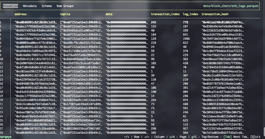
Figure 1: Rows in parqeye. The Visualize tab shows the first rows of eth_logs.parquet.
The metadata tab already tells the first part of the story: 2.74 GiB raw, 1.17 GiB on disk, only 2.35x (Figure 2). For columnar data with this many repeated values, that feels low.
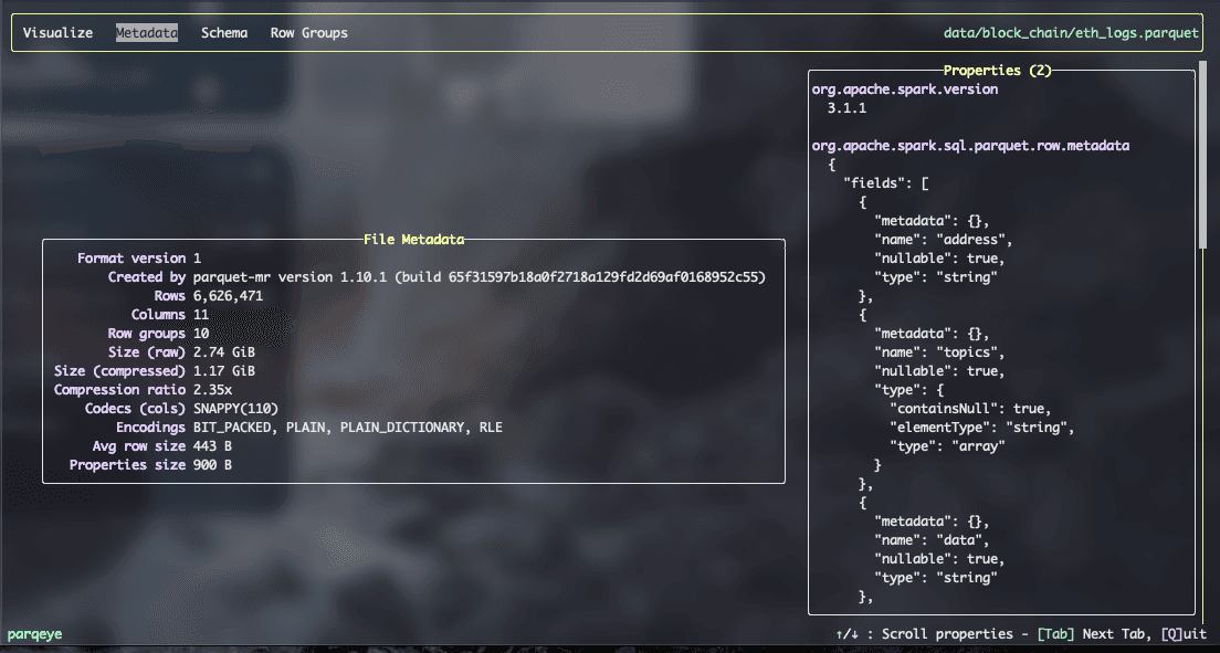
Figure 2: File metadata in parqeye. 2.74 GiB of raw data becomes 1.17 GiB on disk, a compression ratio of only 2.35x.
The schema tab breaks it down per column (Figure 3, Table 2):
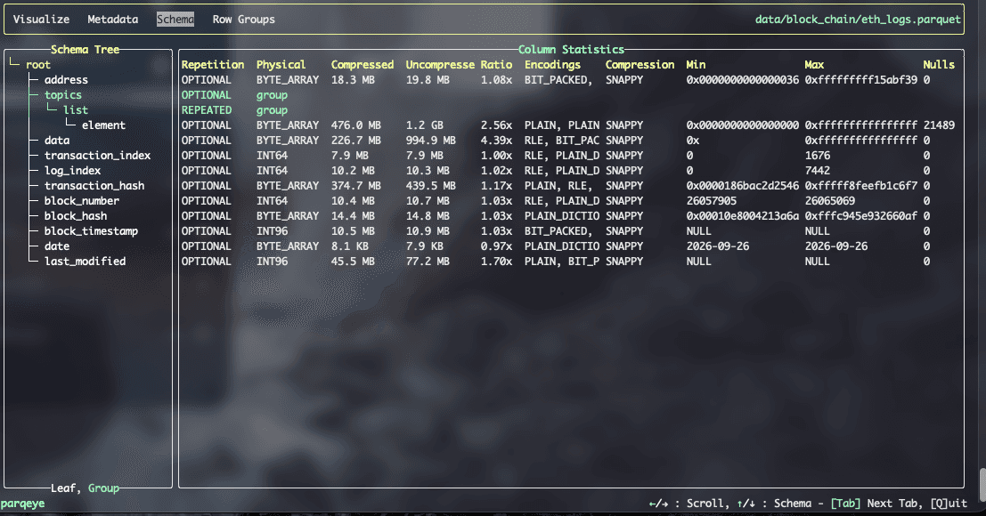
Figure 3: Per-column statistics in parqeye. topics and transaction_hash are the largest columns and compress the least.
Table 2: Compressed and uncompressed size per column of the original file, from parqeye's Schema tab. Three columns hold ~93% of the bytes.
| Column | Compressed | Uncompressed | Ratio |
|---|---|---|---|
topics (list) | 476.0 MB | 1.2 GB | 2.56x |
transaction_hash | 374.7 MB | 439.5 MB | 1.17x |
data | 226.7 MB | 994.9 MB | 4.39x |
last_modified | 45.5 MB | 77.2 MB | 1.70x |
address | 18.3 MB | 19.8 MB | 1.08x |
block_hash | 14.4 MB | 14.8 MB | 1.03x |
block_timestamp | 10.5 MB | 10.9 MB | 1.03x |
log_index | 10.2 MB | 10.3 MB | 1.02x |
block_number | 10.4 MB | 10.7 MB | 1.03x |
transaction_index | 7.9 MB | 7.9 MB | 1.00x |
Three columns (topics, transaction_hash, data) make up ~93% of the file. Notice something odd, though: address has only 59K distinct values in 6.6 M rows and block_number only 7K. They should compress to almost nothing, yet they sit at ~1.03x. Let's dig into the pages.
Dictionary encoding that gives up
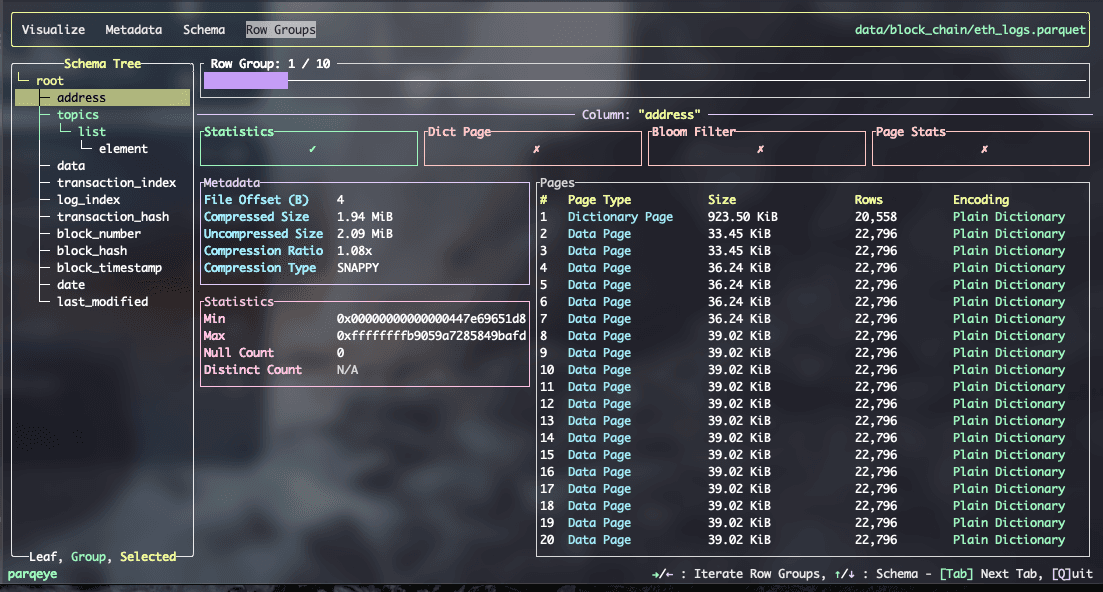
Figure 4: Pages of the address column in the first row group. One 923 KiB dictionary page is followed by small dictionary-encoded data pages.
For address (Figure 4), a 923 KiB dictionary page is followed by data pages of ~36 KiB, each holding 22,796 rows. That is dictionary encoding working as designed: each row becomes a small integer index. But look at topics (Figure 5):
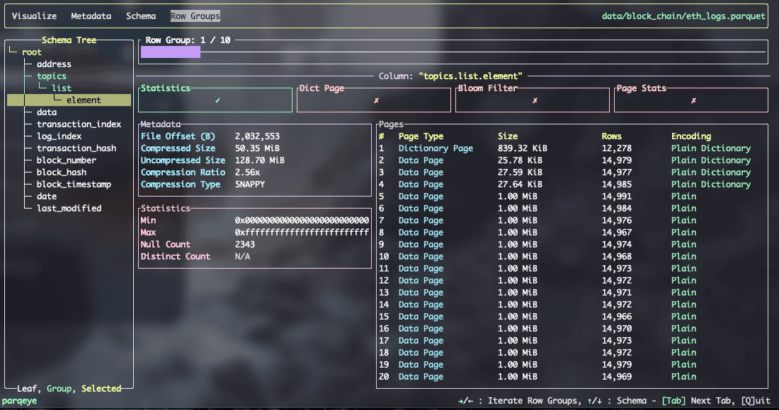
Figure 5: Pages of topics.list.element in the first row group. After a few dictionary-encoded pages, the writer falls back to 1 MiB Plain pages.
The first few data pages use Plain Dictionary, and then it flips to Plain with pages of 1 MiB each. Parquet writers cap the dictionary page size (1 MiB by default). Once the dictionary fills up, the writer falls back to plain encoding for the rest of the column chunk. The same happens for data (Figure 6):
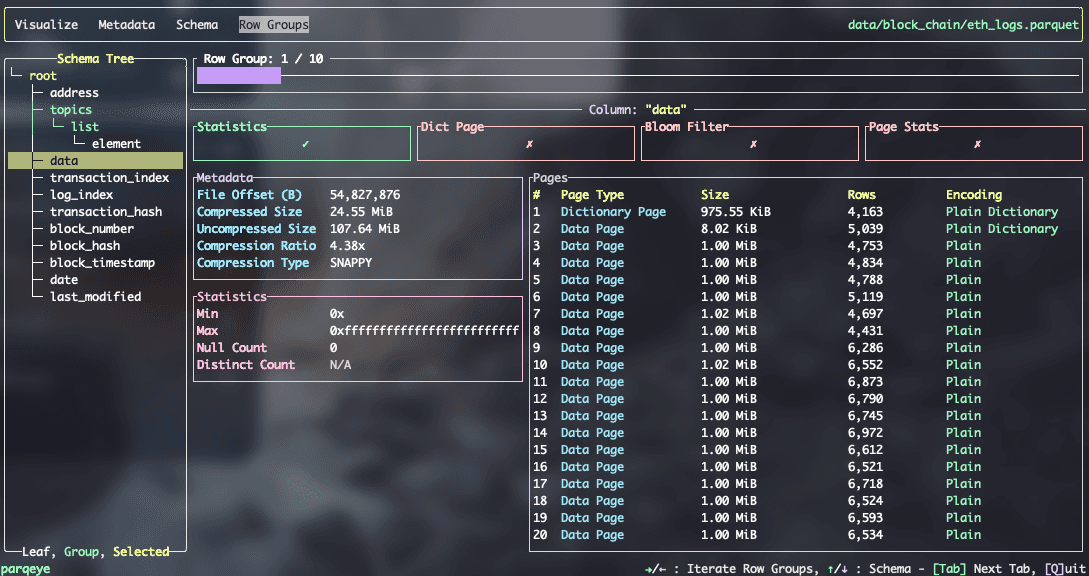
Figure 6: Pages of the data column in the first row group, showing the same fallback from dictionary to Plain encoding.
Two problems compound here:
- Rows are in arbitrary order. Every row group contains logs from all 59K contracts and all 7K blocks. The dictionary is big, the indices are random, and nothing lines up for run-length encoding or for the compressor.
- Values are hex strings. A 32-byte hash stored as
0xplus 64 ASCII characters is twice the size it needs to be, and half of that entropy is wasted on the alphabet.
The same arbitrary ordering has a second cost: min/max statistics become useless, because every row group spans the whole range of every column.
Two experiments
That gives us two questions to test on this file:
- Bloom filters on a high-cardinality column:
transaction_hashis nearly unique, so min/max statistics can't skip anything. Can bloom filters speed up lookups on the file as it is, without rewriting it? - Sort and compress: now we do rewrite the file. How much smaller can it get by changing the codec, the row order and the encoding, and what does that do to queries? We finish by asking whether sorting by hash beats the bloom filter from Experiment 1.
Experiment 1: Bloom filters on a high-cardinality column
Take a point lookup: "show me every log of transaction 0x4b1a...". transaction_hash is nearly unique (~1.09 M values over 6.6 M rows), so there is nothing to cluster. Hashes are random, so every row group's min/max range covers almost any hash and nothing can be skipped: the reader scans all 10 of 10 row groups.
The question for this experiment is whether bloom filters can fix that on the file as it is.
Adding bloom filters to the original file
A bloom filter is a small per-row-group bitmap that answers "is this value definitely not in here?". It needs no sort order, so in theory it fixes exactly the case where min/max stats fail. The interesting question is whether it's worth adding to the original file as it is, without re-sorting anything. (Combining it with a hash sort would be pointless, since sorting already gives each row group a narrow range. Sorting comes up in Experiment 2.)
PyArrow 21 can't write bloom filters, so I used DuckDB 1.5, which can both write them and use them to skip row groups. I kept the original row order and Snappy, and tried two row-group sizes: 700K rows (like the original) and 131K rows. Lookups use SELECT * on 20 existing hashes, and on 20 random hashes that don't exist. Table 3 has the results, and Figures 7 and 8 plot the two lookup cases.
Table 3: Transaction hash lookups on the original row order, with and without bloom filters (DuckDB, Snappy, average of 20 lookups, SELECT *). The filters add 4.8 to 6.3 MB; the size drop comes from raising DuckDB's dictionary limits.
| Layout (original row order, Snappy) | Size | Row groups | Existing hash | Non-existent hash |
|---|---|---|---|---|
| Original file | 1195 MB | 10 | 978 ms | 363 ms |
| Rewritten, no bloom, 700K rows/group | 1185 MB | 10 | 978 ms | 412 ms |
| Bloom 1%, 700K rows/group | 718 MB | 10 | 622 ms | 0.8 ms |
| Rewritten, no bloom, 131K rows/group | 1167 MB | 51 | 540 ms | 364 ms |
| Bloom 1%, 131K rows/group | 819 MB | 51 | 316 ms | 1.7 ms |
Speedup is relative to the original file. DuckDB, average of 20 lookups, SELECT *.
With a bloom filter, every row group is rejected without reading any column data. The bars are so short because there is almost nothing left to read.
Three things to take from this table.
1. Misses become almost free. A hash that isn't in the file drops from ~360-410 ms to under 2 ms, a ~200-500x speedup, because the filter rejects every row group and the reader touches no column data at all. If your workload is "does this transaction exist?" (deduplication, idempotent loads, validation), this is the big win.
2. Hits improve, but modestly (~1.6-1.7x). This surprised me. A transaction has ~6 logs on average, and since the file is not ordered by transaction, those logs are scattered: an average hash appears in 2.6 of 10 row groups (3.3 of 51), so the reader still has to decode those groups even with a perfect filter. Bloom filters can tell you a row group doesn't contain a value; they can't gather the rows that do. Smaller row groups help (316 ms vs 622 ms) because each false hit costs less, at the price of more metadata.
3. The size didn't go down because of bloom filters. The bloom files are much smaller than the original (718 and 819 MB vs ~1.18 GB), but that's not the filters. They add only 4.8 MB (700K rows/group) and 6.3 MB (131K rows/group), about 0.5%. The saving is a side effect: to make DuckDB write filters for every row group I raised its dictionary size limits, which also stopped the dictionary-to-plain fallback we saw in parqeye. topics went from 473 MB to 165 MB and transaction_hash from 369 MB to 183 MB. So the "fix the dictionary fallback" lesson is worth a lot on its own.
That last point is also a catch. My first attempt, with default limits, produced a bloom filter in only 13 of 51 row groups, because DuckDB writes filters only for dictionary-encoded column chunks. The rest had fallen back to PLAIN, so there was nothing to prune and the speedup nearly vanished. Always verify with parquet_metadata() that the filters exist in every row group.
Sorting by transaction_hash (covered in Experiment 2) can beat this for hits, because all of a transaction's logs then sit together in one row group. Bloom filters can't do that. But they cost 0.5% instead of a full rewrite with a new sort order, they need no change to the data layout, and they make misses free.
Limits to keep in mind:
- Engine support: PyArrow wrote no filters and, as far as I could tell, doesn't prune with them. DuckDB, Spark and Trino (with the right settings) do.
- Only equality lookups: bloom filters don't help range predicates or low-cardinality columns. Use them for hashes and IDs.
- Tiny data hides the benefit: at 1 GB on a local SSD, even a full scan takes about a second. On object storage, skipping a row group means skipping a network request, which is where the miss case turns into real money.
Experiment 2: Sort and compress
Experiment 1 left the file untouched. This one rewrites it, with a smaller file as the goal and then a look at what the new layout does to queries. I re-wrote the file with PyArrow in a handful of variants. I dropped last_modified (an ingestion timestamp that nobody queries by), so all variants below cover the same 10 columns. The variants change one thing at a time (Table 4):
Table 4: File size for each write variant, changing one thing at a time (PyArrow, 1 M-row groups, last_modified dropped).
| Variant | What changed | Size | vs baseline |
|---|---|---|---|
| a. Snappy | Baseline rewrite, 1 M-row groups | 1161 MB | 1.0x |
| b. ZSTD level 3 | Codec only | 539 MB | 2.2x |
| c. ZSTD level 9 | Heavier codec | 519 MB | 2.2x |
| d. Sorted + ZSTD 3 | Sort by address, block_number, log_index | 265 MB | 4.4x |
| e. Sorted + binary + ZSTD 3 | Hex strings stored as raw bytes | 226 MB | 5.1x |
| f. Sorted + binary + ZSTD 9 | Heavier codec on top | 218 MB | 5.3x |
import pyarrow.parquet as pq

t = pq.read_table('eth_logs.parquet')
t = t.sort_by([('address', 'ascending'),
               ('block_number', 'ascending'),
               ('log_index', 'ascending')])
pq.write_table(t, 'eth_logs_sorted.parquet',
               compression='zstd', compression_level=3,
               row_group_size=1 << 20)
A few lessons stand out.
1. The codec is worth a 2x, and level barely matters. Going from Snappy to ZSTD roughly halves the file. Going from ZSTD 3 to 9 buys under 4% while taking about 2.6x longer to write (8 s → 21 s). Snappy optimizes for speed, ZSTD for ratio; for data that is written once and read many times, ZSTD level 3 is an easy default.
2. Sorting is worth another 2x, and it costs nothing at read time. This is the biggest single lever. Same codec, same data, only the row order changed (Table 5):
Table 5: Compressed size per column with ZSTD level 3, unsorted versus sorted by address, block_number, log_index. Every column shrinks, the repeated ones most of all.
| Column | ZSTD 3 (unsorted) | ZSTD 3 (sorted) | Saving |
|---|---|---|---|
address | 15.2 MB | 1.5 MB | 10x |
block_number | 10.3 MB | 3.0 MB | 3.4x |
block_timestamp | 10.5 MB | 3.2 MB | 3.3x |
block_hash | 11.9 MB | 4.6 MB | 2.6x |
transaction_hash | 161.3 MB | 82.9 MB | 1.9x |
topics | 195.6 MB | 88.0 MB | 2.2x |
data | 116.1 MB | 70.7 MB | 1.6x |
Sorting by address turns that column into a handful of very long runs, and RLE collapses it to ~1.5 MB. Within one contract, logs tend to look alike (the same event signatures in topics, similar payloads in data), so even the "random-looking" columns compress better once similar rows sit next to each other. This is the same reason clustering keys and sort orders matter in warehouses.
3. Hex-as-binary gives a final ~15%. Storing address, hashes, topics and data as raw bytes (bytes.fromhex) shaved another 39 MB off the sorted file. Less than I expected, because ZSTD and dictionary encoding already squeeze most of the redundancy out of hex text. But it also halves the in-memory footprint after decoding, which matters for engines that materialize strings. The trade-off is readability: you now need hex() in every query.
4. Some columns are just incompressible. transaction_hash is 32 random bytes per transaction. Even sorted, it takes 74–83 MB, about a third of the best file. That is entropy, not inefficiency. If you don't need it for a given analysis, don't read it. Column projection, covered below, is how you avoid paying for it.
What the sorted layout does to queries
Compression is only half of the story; the other half is how much data a query must touch. Take a typical question: "give me all USDC logs" (address = 0xa0b8...eb48, 633,956 rows).
Original layout. address min/max per row group spans 0x00... to 0xff... in every one of the 10 row groups. Parquet stores these statistics so that readers can skip row groups that cannot match, but here none can be skipped: all 10 of 10 have to be read.
Sorted layout. Because rows are ordered by address, each row group covers a narrow address range. The USDC filter touches 1 of 7 row groups.
Table 6: Query times on the original and the sorted file (PyArrow, best of 3, warm cache, local SSD). Sorting by address speeds up address queries and slightly slows block-range queries.
| Query (PyArrow, warm cache, laptop) | Original | Sorted + ZSTD |
|---|---|---|
| Read everything, no filter | 0.74s | – |
address = USDC, 2 columns | 0.05s | 0.02s |
address = USDC, all columns | 0.37s | 0.14s |
block_number in a 300-block range, 2 cols | 0.04s | 0.06s |
Read the numbers in Table 6 with care. They're best-of-3 on a warm page cache on a local SSD, and the data is only 1 GB. On object storage such as S3 you pay per byte and per request, so bytes skipped matters much more than the wall-clock times above.
Three takeaways:
- Column projection is the cheapest optimization. Asking for 2 columns instead of 10 took the USDC query from 0.37 s to 0.05 s on the original file, with no rewrite at all. This is the whole point of a columnar format.
SELECT *throws it away. - Sort order is a bet on your query pattern. The sort by
addresshelped the address query (0.37 s → 0.14 s on all columns, and 1 of 7 row groups read instead of 10 of 10) but made the block range query slightly slower (0.04 s → 0.06 s). Both layouts have to scan for a block range, but after sorting by address, the matching blocks are scattered across every contract's run, so the reader has to touch more pages. If most of your queries slice by time, sort byblock_numberfirst; if they slice by contract, sort byaddress. You can't have both for free, but partitioning or a Z-order style layout can approximate it. - Row group size is a knob, not a constant. Small row groups mean more effective pruning but more metadata and less compression per group; large ones mean the opposite. I used 1 M rows here; production tables often land between 128 MB and 1 GB per group.
Sorting by transaction_hash instead of using bloom filters
Back to the hash lookup from Experiment 1. The other way to fix it is to re-sort the file. I picked 5 random hashes and ran the same equality filter against three layouts (Table 7). This uses PyArrow, so the numbers are not directly comparable with the DuckDB bloom results above:
Table 7: Transaction hash lookup across three layouts (PyArrow, average of 5 random hashes, ZSTD 3 for the rewritten files). Only the hash-sorted file lets the reader skip row groups.
| Layout | Size | Avg lookup | Row groups read |
|---|---|---|---|
| Original (Snappy, unsorted) | 1195 MB | 0.87 s | 10 / 10 |
Sorted by address | 265 MB | 0.75 s | 7 / 7 |
Sorted by transaction_hash | 302 MB | 0.03 s | 1 / 26 |
Sorting by address gives essentially no benefit here: hashes are random, so every row group's min/max range covers almost any hash and nothing can be skipped. Sorting by transaction_hash makes each row group cover a narrow, non-overlapping range, so the reader jumps straight to one row group (a ~27x speedup, with smaller 256K-row groups).
There is no free lunch, though:
- Only one leading sort key. Sorting by hash lands at 302 MB instead of 265 MB (+14%), because we lost the address clustering that helped compression. And the USDC query is back to scanning everything.
- Options when you need both: keep two copies of the table sorted differently (storage is cheap, scans aren't), or keep one copy and build a small lookup table
transaction_hash → block_numberso hash lookups become block-range queries. Bloom filters, covered above, are the third option. - Range stats are useless for random keys. Min/max is only as good as the sort order behind it, which is why "hash lookups on an address-sorted file" behave like a full scan.
Combining both: sort by address, bloom filter on the hash
Sorting and bloom filters solve different problems, so they don't have to compete. Sorting by address gives the compression and the contract queries. A bloom filter on transaction_hash then covers the point lookups that the sort can't. This is different from adding a filter to a hash-sorted file, which would be pointless.
Table 8: Hash lookups on the address-sorted file, with and without a bloom filter on transaction_hash and address (DuckDB, ZSTD, 131K rows per row group, 51 groups, average of 20 lookups). The filter adds about 2 MB. The two files came from different writers (PyArrow and DuckDB), so treat small differences with caution.
| Layout | Size | Existing hash | Non-existent hash |
|---|---|---|---|
| Original file | 1195 MB | 540 ms | 61 ms |
Sorted by address, no bloom filter | 263 MB | 53 ms | 46 ms |
Sorted by address, bloom filter | 265 MB | 27 ms | 2.3 ms |
The address sort alone already cuts a hash lookup by about 10x here. Hashes are still random, so it isn't pruning row groups, and I did not isolate why it is faster: the rewritten file also uses ZSTD, smaller row groups and dictionary encoding, so treat that 10x as a property of this file, not of sorting. The bloom filter then halves the hit time and makes misses about 20x faster, for under 1% more space. The filter on address itself adds only 0.1 MB and little benefit here, because the sort already gives tight min/max ranges.
A gap in these experiments: I only benchmarked a bloom filter on transaction_hash. I did not test one on address in the unsorted file, or filters on several columns at once.
Takeaways
Sorting and bloom filters do different jobs.
- Sorting buys compression and range pruning, but commits you to one access pattern. It gave a ~2x size reduction and made min/max statistics prune row groups. It works for equality and range predicates, but you get one leading key. Choose it from your queries:
addressfor contract queries,transaction_hashfor point lookups. Whatever you didn't sort by gets no help, and can get slightly worse (the block-range query did). - Bloom filters buy point-lookup pruning on any column without committing you to a layout. They cost about 0.5% per column, work on the file as it is, and can be added for several columns. Misses became ~200-500x faster and hits ~1.7x faster. But they only help equality, they only rule row groups out (so scattered hits still cost a read), they do nothing for compression, and they need an engine that reads them.
- Use both when you have both patterns. Sort by the column you filter and range-scan on, and add bloom filters to the high-cardinality columns you look up by equality. On the address-sorted file, a filter on the hash halved hit time and cut misses ~20x for about 2 MB.
Along the way:
- Look at the file before tuning the query. One
parqeyesession showed that three columns were 93% of the bytes and that dictionary encoding was silently falling back to plain. - Fix the dictionary fallback. Raising the dictionary limit cut
topicsfrom 473 to 165 MB andtransaction_hashfrom 369 to 183 MB, and it is also what lets bloom filters exist in every row group. Verify withparquet_metadata(). - Pick ZSTD over Snappy for write-once data. Level 3 gets you nearly all of the benefit.
- Don't store binary data as hex text, but expect a modest win, not a miracle.
- Never read columns you don't need. It's the cheapest optimization you'll ever make.
Together: 1.16 GB → 218 MB (5.3x) with a few lines of PyArrow and no change to the data itself, plus near-free "does this hash exist?" checks from a ~0.5% bloom filter. And this is one day of logs; Ethereum has years of them.
Caveats: single machine, warm cache, one day of data, and a single query pattern per test. The two experiments use different engines (DuckDB for bloom filters, PyArrow for compression and sorting), so compare numbers within an experiment, not across them. I tested bloom filters on one high-cardinality column only. Treat the ratios as directional, and rerun on your own data.